

How Quantitative Tightening (QT) Impacts US Equity Liquidity?
Summary Paragraph
Quantitative Tightening (QT) is a monetary policy tool where a central bank, such as the Federal Reserve, reduces the size of its balance sheet by selling government bonds or allowing them to mature without reinvesting the proceeds.
This is the direct opposite of Quantitative Easing (QE), which involves purchasing assets to inject liquidity into the financial system.
The primary goal of QT is to curb inflation and normalise monetary policy, but its execution directly contracts liquidity, impacting all asset classes.
To fully grasp the current market environment, one must understand the monumental shift from an era of accommodative monetary policy to one of constraint.
For over a decade, global markets were buoyed by Quantitative Easing (QE), a policy that became synonymous with asset price inflation. Now, the tide has turned.
As a market analyst, my focus is on dissecting the mechanics and ramifications of this reversal, a process known as Quantitative Tightening (QT).
From QE to QT: Understanding the Fed’s Balance Sheet Policies
The journey from QE to QT began after the 2008 financial crisis. To avert a systemic collapse, the Federal Reserve initiated large-scale asset purchases, primarily US Treasuries and mortgage-backed securities (MBS).
This action, QE, swelled its balance sheet from under $1 trillion to nearly $9 trillion by its peak. The objective was to lower long-term interest rates, encourage borrowing and investment, and inject liquidity directly into the banking system.
This liquidity found its way into financial assets, including equities, driving one of the longest bull markets in history.
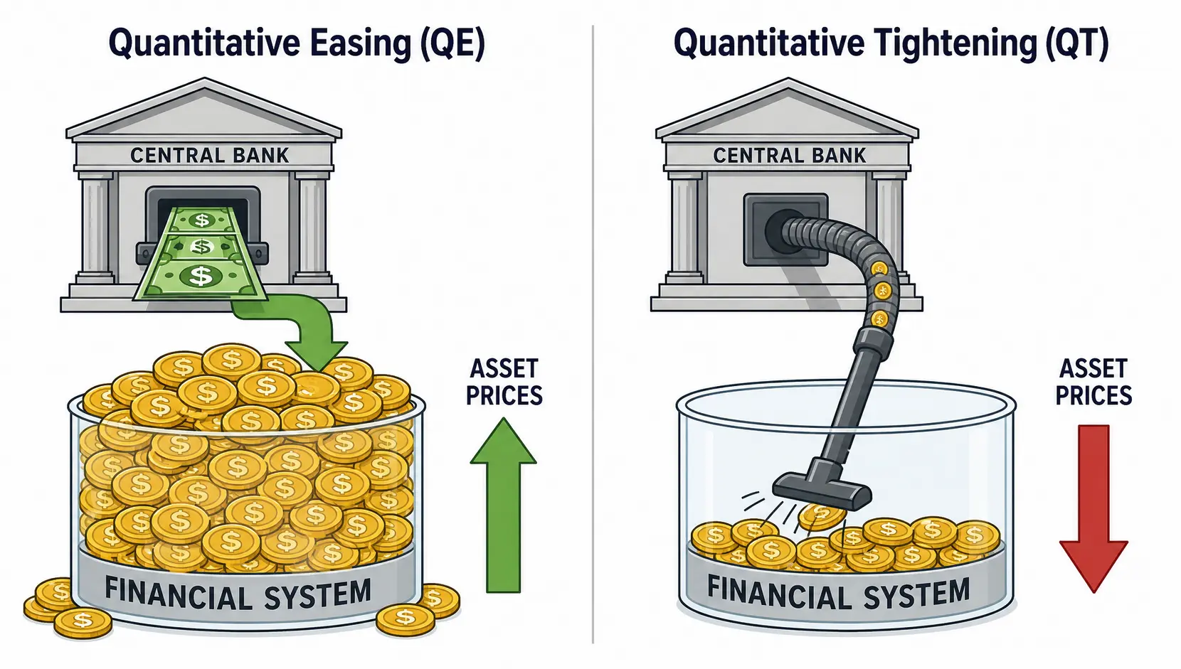
By 2022-2023, with inflation running at multi-decade highs, the Fed’s mandate shifted. It pivoted to QT to remove the excess liquidity and cool the overheating economy.
The process is mechanical: the Fed sets a monthly cap on the amount of maturing securities it will allow to ‘run off’ its balance sheet without reinvestment.
This forces the US Treasury to find other buyers for its debt, effectively pulling cash (liquidity) out of the private sector.
The Core Mechanism: How QT Removes Liquidity from the Financial System
When the Fed’s assets decrease, its liabilities must also decrease. These liabilities are primarily composed of commercial bank reserves held at the Fed and the Treasury General Account (TGA).
As bonds mature and are not replaced:
- The US Treasury redeems the maturing bond, transferring cash to the Fed.
- This cash is often drawn from tax receipts or by issuing new bonds to the public.
- When private entities (like investment funds or individuals) buy these new bonds, they use cash from their commercial bank accounts.
- This action drains reserves from the commercial banking system, reducing the overall ‘monetary base’.
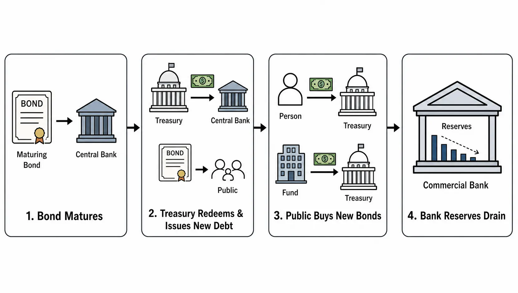
This reduction in bank reserves is the lynchpin of QT’s impact. Fewer reserves mean banks have less capacity for lending and market-making activities, leading to a contraction in overall credit and liquidity available to the economy and, by extension, the equity markets.
| Feature | Quantitative Easing (QE) | Quantitative Tightening (QT) |
|---|---|---|
| Objective | Stimulate economy, lower long-term rates | Curb inflation, normalise policy |
| Fed’s Action | Buys government bonds & MBS | Sells bonds or lets them mature |
| Impact on Balance Sheet | Expands | Contracts |
| Effect on Liquidity | Injects liquidity (increases bank reserves) | Removes liquidity (drains bank reserves) |
| Typical Market Impact | Lower yields, higher asset prices, ‘risk-on’ | Higher yields, pressure on asset prices, ‘risk-off’ |
The Direct Impact of QT on US Equity Market Liquidity and Volatility
Pro Tip
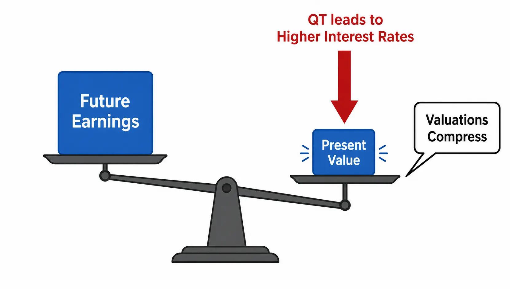
The primary transmission mechanism from QT to equities is through the ‘discount rate’ and ‘liquidity premium’. As QT pushes benchmark interest rates higher, the discount rate used to value future corporate earnings rises, immediately compressing stock valuations.
Simultaneously, reduced market liquidity means investors demand a higher premium for holding less liquid assets, further pressuring stock prices downwards.
Analyzing the Effect on Stock Valuations and Price Multiples
The valuation of any stock is, at its core, the present value of its expected future cash flows.
The formula for this calculation uses a discount rate, which is heavily influenced by the ‘risk-free’ rate, typically the yield on US Treasury bonds. QT puts direct upward pressure on these yields.
When the Fed steps away as a major buyer, the Treasury must offer higher yields to attract private capital.
As the risk-free rate rises, the discount rate used in equity valuation models also increases. A higher discount rate means future earnings are worth less in today’s terms, causing price-to-earnings (P/E) multiples to contract.
During the era of QE and zero interest rates, high P/E multiples were justifiable. In a QT environment, a P/E of 30x may contract to 20x or even 15x, even if the company’s earnings forecast remains unchanged.
This is a mathematical certainty that traders must respect.
The Link Between Shrinking Bank Reserves and Equity Market Volatility
Liquidity is the bedrock of market stability. When it is abundant, trades are executed smoothly with minimal price impact (low ‘spread’). When liquidity vanishes, spreads widen, and even small orders can cause significant price swings. This is the definition of volatility.
QT’s draining of bank reserves directly impairs the ability of primary dealers and market makers to facilitate smooth trading. With less capital on their balance sheets, these institutions are less willing to hold inventory or absorb large client orders.
This fragility was starkly demonstrated during the brief but intense market convulsions of 2022 and 2024. The CBOE Volatility Index (VIX), often called the market’s ‘fear gauge’, has shown a clear tendency to spike during periods of accelerated QT as market depth deteriorates.
For traders, this means wider bid-ask spreads, increased slippage, and a greater risk of flash crashes in individual stocks or the broader market.
Risk Warning: The Illusion of Liquidity
Market participants must be wary of the ‘illusion of liquidity’. In modern electronic markets, liquidity can appear deep on screen but evaporate instantaneously under stress.
During a QT-induced liquidity event, the ability to sell assets at a fair price may disappear, forcing panic-selling and exacerbating a downturn. This is a systemic risk that cannot be diversified away easily.
Broader Market Risks: Could Quantitative Tightening Trigger a Financial Crisis?
Summary Paragraph
Yes, if managed improperly, QT can significantly elevate the risk of a financial crisis. The primary threat lies in the plumbing of the financial system, specifically the repo market, where a shortage of bank reserves can cause funding stresses to spiral out of control.
Furthermore, the relentless upward pressure on interest rates can expose vulnerabilities in heavily indebted corporations and even sovereign nations, creating a feedback loop of credit defaults and market panic.
Examining the Risk of a Liquidity Crisis in the Repo Market
The repurchase agreement (repo) market is a critical but often overlooked part of the financial system. It is where financial institutions lend to each other overnight, using government securities as collateral.
It is the essential lubricant for the global financial machine. This market depends entirely on the availability of ample bank reserves.
The 2019 repo market spike serves as a crucial case study. As the Fed was then conducting a much smaller-scale QT, bank reserves fell below a critical level.
This scarcity caused overnight lending rates to surge dramatically, forcing the Fed to intervene with emergency liquidity injections. The current, more aggressive QT cycle running into 2026 presents a far greater risk.
A seizure in the repo market would be catastrophic, as it would halt the ability of dealers to finance their operations, leading to forced asset sales and a potential systemic crisis far more rapid than the 2008 collapse.
How QT Puts Upward Pressure on Interest Rates and Bond Yields
The relationship between QT and interest rates is direct and unambiguous. By ceasing to be the buyer of last resort for government debt, the Fed forces the market to absorb trillions of dollars in new Treasury issuance.
To entice buyers, yields must rise. This has several second-order effects:
- Increased Corporate Borrowing Costs: Corporations price their debt off the Treasury yield curve. Higher government bond yields translate directly to higher borrowing costs for companies, squeezing profit margins and reducing funds available for buybacks and dividends.
- Mortgage Rates and Housing: Rates for consumer loans, particularly mortgages, are tied to the yield on MBS and Treasuries. QT has been a primary driver of the surge in mortgage rates, cooling the housing market and impacting consumer wealth.
- The ‘Crowding Out’ Effect: As capital flows into newly attractive, higher-yielding government bonds, it is ‘crowded out’ from riskier assets like stocks. This rotation from equities to bonds is a classic feature of a tightening cycle.
| Market Indicator | QE Environment (Low Rates) | QT Environment (Rising Rates) |
|---|---|---|
| Risk-Free Rate (e.g., 10-Yr Treasury) | Low / Suppressed | High / Rising |
| Equity Valuations (P/E Ratios) | Expanded / High | Compressed / Low |
| Investor Risk Appetite | High (‘Risk-On’) | Low (‘Risk-Off’) |
| Market Volatility (VIX) | Generally Low / Subdued | Elevated / Prone to Spikes |
| Credit Spreads | Tight | Widening |
Frequently Asked Questions
1. What is the main difference between Quantitative Easing (QE) and Quantitative Tightening (QT)?
From a practical standpoint, QE is the act of a central bank printing new money to buy assets, which expands its balance sheet and injects liquidity into the banking system. Think of it as pressing the accelerator on the economy.
QT is the opposite; the central bank removes money from the system by letting those assets mature or selling them, shrinking its balance sheet. This is akin to applying the brakes.
2. How does quantitative tightening affect the average investor?
For the average investor, QT’s effects are felt in three main ways. First, it generally leads to lower stock market returns as valuations compress.
Second, it increases market volatility, meaning more frequent and larger price swings in your portfolio. Third, it pushes up interest rates on savings accounts and bonds, making these ‘safer’ assets more attractive relative to equities.
It fundamentally alters the risk-reward calculation for your entire investment portfolio.
3. What are the historical examples of QT’s impact on the stock market?
The most relevant example is the Fed’s first attempt at QT from 2017-2019. During that period, particularly in the fourth quarter of 2018, the S&P 500 fell nearly 20% as the pace of QT accelerated.
The market only bottomed and recovered after the Fed signalled a pivot away from tightening.
Another key event was the September 2019 repo market crisis, which showed how draining liquidity could destabilise the core financial plumbing, forcing the Fed to abruptly end QT and restart balance sheet expansion.
4. Which stock sectors are most vulnerable during QT?
Typically, the sectors that benefit most from QE are the most vulnerable to QT.
This includes high-growth technology stocks with long-duration cash flows (their valuations are highly sensitive to rising discount rates), speculative ‘meme stocks’, and unprofitable companies that rely on cheap capital to survive.
Conversely, sectors like consumer staples, healthcare, and utilities, which have more stable earnings, tend to be more resilient.
5. Can the Federal Reserve control the impact of QT?
To an extent, yes, but it’s an imprecise science. The Fed can adjust the pace of its balance sheet runoff by changing the monthly caps.
It has also established facilities like the Standing Repo Facility (SRF) to act as a safety valve if funding markets seize up.
However, the exact level of bank reserves required for the system to function smoothly is unknown. This means the Fed is effectively navigating in the dark, and the risk of a policy misstep—tightening too much, too fast—remains elevated.
Andrew Wong’s Final Thoughts
Market movements are a combination of macroeconomic gravity and technical psychology. For the past fifteen years, the gravity has been artificially suspended by Quantitative Easing.
Now, with Quantitative Tightening, the full weight of normalised interest rates and reduced liquidity is being reapplied. The psychological shift from a ‘buy the dip’ mentality to a ‘sell the rip’ environment is a direct consequence.
As we move through 2026, the key to successful navigation is not to predict the exact timing of market moves, but to understand the immense gravitational force that QT exerts on all asset classes.
Acknowledging this new reality and adjusting risk exposure accordingly is the only prudent path forward.
Sources & Methodology
Andrew Wong strictly relies on primary regulatory data and authoritative official information to ensure accuracy. Data cited in this guide is sourced from:
- Federal Reserve Board: Trends in the Size and Composition of the Balance Sheet
- Investopedia: Quantitative Tightening (QT) Definition
- Bank for International Settlements (BIS): September 2019 Repo Market Turmoil Analysis
- Securities Commission Malaysia (SC) – Market Oversight
- Bank Negara Malaysia (BNM) – Financial Stability Review
*Disclaimer: The content of this article represents the personal views of the author (Andrew Wong) and is for educational and reference purposes only. It does not constitute professional investment or financial advice. Trading and investing involve significant risk; proceed with caution.*
